How to Add Drop Down List in Excel (Easy Step-by-Step)

Quick answer: To add a drop-down list in Excel, select the cell, go to Data > Data Validation, and choose List under Allow. Type your items in the Source box (separated by commas) or select a cell range, then click OK. A small arrow appears in the cell, and you can pick from your choices.

Learning how to add drop down list in excel fixes that in about a minute, and I’ll show you every method I use, from the basics to dynamic and dependent lists.

Let’s dive in.

What Is a Drop-Down List in Excel, and Why Should You Use One?

A drop-down list is a small arrow inside a cell that lets you pick from a fixed set of choices instead of typing. It’s built on a feature called data validation, which controls what people are allowed to enter. Honestly, it’s one of the most underrated tools in the whole program, and once you try it, you’ll want it everywhere.

Here’s what you get:

Consistent data entry, so filters and pivot tables actually work
Fewer typos and fewer broken formulas
Cleaner forms, trackers, and dashboards

Microsoft explains that restricting a cell to list choices makes data entry quicker and more accurate. Want to go deeper on the feature itself? See my Excel data validation guide.

How to Add Drop Down List in Excel: Step-by-Step

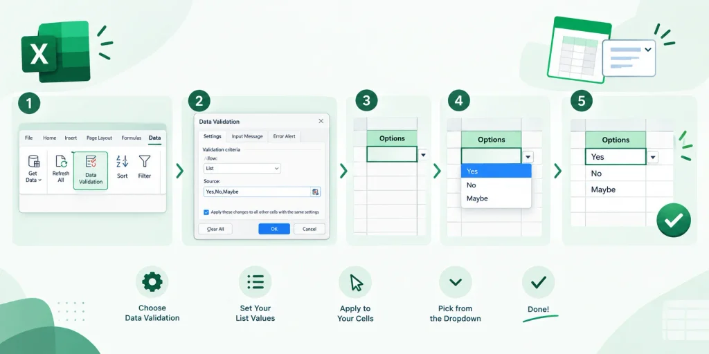
Every drop-down in Excel runs on the same few clicks. Once you know them, every other method in this guide is just a small variation. So let me show you the three foundations first: typed items, a cell range, and an Excel Table. Pick the one that matches your situation, and follow the numbered steps.

Method 1: Type Your Items Directly

This is the fastest option, and it’s perfect for short lists that rarely change, like Yes/No or Low/Medium/High. You don’t need a separate list on your sheet. I use it constantly for quick trackers, and it takes about ten seconds.

Select the cell or range where you want the list.
Click Data > Data Validation.
Under Allow, choose List.
In the Source box, type your items separated by commas, like this: Yes, No, Maybe.
Make sure In-cell dropdown is ticked, then click OK.

The University of Michigan’s IT knowledge base documents the same steps, so it’s not just me saying it.

Method 2: Use a Cell Range or Named Range

Typing works until your list hits 30 entries. Then it’s painful. A better move is keeping your choices in a column, ideally on a separate sheet, and pointing the drop-down at it. That way your list is easy to edit and hard to overwrite by accident. Plus, a named range like =StatusList is far easier to read than a long cell address.

Type your items in one column, with no blank cells.
Select the cells that need the drop-down.
Open Data > Data Validation and choose List.
Click the Source box and select your list range.
Optionally, name the range and type =StatusList instead.

Method 3: Use an Excel Table (My Favorite)

Want a list that updates itself? This is the one. Microsoft recommends keeping list items in an Excel table, and pressing Ctrl+T converts any range into one. Add a new item at the bottom, and the drop-down picks it up. Zero maintenance.

Xelplus notes that new items added to the table show up without touching your validation settings again.

Select your list and press Ctrl+T.
Name the table something sensible.
Create your drop-down and select the table column as the Source.
Add a new row to the table and test it.

Want to practice? Download the free practice workbook.

Which Drop-Down Method Should You Choose?

Four methods, four different strengths. Rather than guess, compare them side by side. This quick table shows how each one handles setup time, automatic updates, and version requirements. Use it as your cheat sheet whenever you’re building a new list. If you’re unsure, start with the Excel Table method, because it balances simplicity and flexibility best.

Method	Setup Time	Updates Automatically?	Best For	Excel Version
Typed items	Under 15 seconds	No	Short, fixed lists (Yes/No)	All versions
Cell or named range	About 1 minute	No (unless you edit the range)	Medium lists on a separate sheet	All versions
Excel Table	About 2 minutes	Yes, when you add rows	Lists that grow over time	2016 and later
Dynamic UNIQUE list	About 3 minutes	Yes, from source data	Removing duplicates automatically	Microsoft 365 / 2021+

How Do You Make a Drop-Down List From Another Sheet?

This is one of the most common questions, and the answer is refreshingly simple. Keeping your source list on a different sheet is smart, because it protects your choices from accidental edits. You still follow the same Data Validation steps; the only difference is where you click when selecting the Source range.

Type your list on a second sheet (for example, “Lists”).
Go back to your main sheet and select the target cells.
Open Data > Data Validation and choose List.
Click the Source box, switch to the “Lists” tab, and select your items.
Click OK.

Groovypost’s walkthrough shows this exact setup, listing options on another worksheet. And if you want tidy formulas, give the range a name first.

How Do You Add an Input Message and Error Alert?

Creating the list is only half the job. What happens when someone ignores your options and types random stuff? That’s where two extra tabs in the Data Validation window come in. They guide people before they type and stop them after they slip up. Think of them as friendly guardrails for your spreadsheet.

Open Data > Data Validation and click the Input Message tab.
Add a short tip, like “Pick a status from the list.”
Switch to the Error Alert tab.
Choose Stop to block bad entries, or Warning to allow them with a nudge.
Write a clear message and click OK.

According to Microsoft, you can specify your own error message for invalid entries. Use that power wisely.

How Do You Create a Dynamic Drop-Down List With UNIQUE?

Here’s where things get fun. If you use Microsoft 365 or Excel 2021, you can build a dynamic drop-down list that cleans itself. Picture a sales sheet with the same region typed 500 times. You don’t want 500 options; you want each region once. The UNIQUE function handles that, and dynamic array formulas keep the list current.

In an empty cell, type =SORT(UNIQUE(A2:A100)) and press Enter.
The results spill down the column, creating a spill range.
Select your drop-down cell and open Data Validation.
Choose List, then type the cell address followed by a hash, like =$E$2#.
Click OK.

That hash is the spill operator. Excel Campus recommends it over a fixed range, because the validation updates as items are added or removed.

One catch, though. Excel Insider points out that Data Validation doesn’t accept dynamic array formulas directly in the Source box, so spill the formula into cells first. Also, leave empty space below it, or you’ll see a #SPILL! error.

How Do You Build a Dependent Drop-Down List?

Ever wanted a second list that changes based on the first? Pick “USA,” and you get states. Pick “Canada,” and you get provinces. That’s a dependent drop-down list, also called a cascading drop-down. It looks advanced, but the logic is simple: the second list checks the first cell and shows only matching options. Here are two ways to build it. For more lookup tricks, check my XLOOKUP guide.

The Classic Way: INDIRECT and Named Ranges

This is the older method, and it’s been around for years. You create one named range per category, then use the INDIRECT function to convert the first cell’s value into a range name. Microsoft’s community experts describe this exact approach.

Create your first drop-down (for example, countries).
Name each list of dependents exactly like the matching country. Use underscores instead of spaces.
Select the second cell and open Data Validation.
Choose List and type =INDIRECT(A2) as the Source.

The Modern Way: FILTER and XLOOKUP

Prefer skipping named ranges? Me too, most days. FILTER and XLOOKUP pull matching items straight from your dataset, so everything stays in one place. Chandoo shows XLOOKUP returning a category’s column and feeding it to the validation rule, and Contextures demonstrates a FILTER-based version.

Build your first list with UNIQUE.
Write a FILTER or XLOOKUP formula that reacts to that selection.
Point the second drop-down at the resulting spill range.

Writing those formulas from scratch can feel intimidating. If that’s you, an AI Excel formula generator like Formulaizer can draft a FILTER or XLOOKUP formula from a plain-English description. Just test the result on sample data before you rely on it.

How Do You Color-Code a Drop-Down List?

A plain list works fine. But a green “Done” and a red “Blocked” is much easier to scan at a glance. Here’s the surprise, though: data validation can’t change colors by itself. You need conditional formatting, which is a separate feature that pairs perfectly with your list. I add it to almost every project tracker I build.

Select the cells that contain your drop-down.
Go to Home > Conditional Formatting > New Rule.
Choose Format only cells that contain.
Set Cell Value, equal to, and type the item (for example, =”Done”).
Click Format, pick a fill color, then click OK.
Repeat for every item in your list.

The Microsoft Community Hub walks through a red, yellow, and green example. For a full status drop-down tutorial, see Excel Insider’s color guide.

Can You Select Multiple Items in One Cell?

Short answer: not natively. A standard list allows one choice per cell, which surprised me too the first time. If you truly need a multi-select drop-down, you’ll need a small VBA macro that runs whenever the cell changes and adds the new choice to the old one. It works, but it’s a bit fragile, so I only recommend it when you really need it.

A Microsoft Q&A thread shares a widely used Worksheet_Change macro, credited to Sumit Bansal of TrumpExcel.

Save your file as .xlsm so the macro survives.
Test on a copy first, since macro changes are hard to undo.
Consider separate columns instead of one crowded cell.

Why Is My Excel Drop-Down Arrow Missing?

Sometimes you follow every step and the arrow refuses to show up. Don’t panic. In my experience, three settings cause almost every problem, and none of them require rebuilding your list. Work through these fixes in order, starting with the most common one.

Fix 1: Turn on the In-cell dropdown option. When this box is unchecked, the arrow disappears, but the rule still restricts entries, as Spreadsheet Planet explains. Select the cells, open Data Validation, tick In-cell dropdown, and click OK.

Fix 2: Show objects. Go to File > Options > Advanced and set “For objects, show” to All, as Microsoft Community Hub contributors suggest.

Fix 3: Unlock cells on protected sheets. Excel Insider recommends unlocking drop-down cells (press Ctrl+1, open the Protection tab, uncheck Locked) before reapplying protection.

Frequently Asked Questions About Excel Drop-Down Lists

Does the drop-down list work in Excel for the web and Mac?

Yes. Microsoft’s guide lists Excel for Mac among the supported versions, and its data validation article says the functionality is the same in Excel for the web. Menu names may vary slightly, so look for Data Validation on the Data tab.

How do I edit a drop-down list?

Select the cell, open Data > Data Validation, and change the Source box. If your list lives in a range or table, simply edit the items there. The drop-down updates to match.

How do I remove a drop-down list?

Select the cells, open Data > Data Validation, click Clear All, then click OK. Microsoft confirms this removes the validation from those cells.

Is right-click “Pick From Drop-down List” the same thing?

Nope. That option only offers values already typed in the cells above, as a Microsoft Community Hub reply explains. A real drop-down needs Data Validation.

Final Thoughts on How to Add Drop Down List in Excel

So there you have it.

You now know how to add drop down list in excel using typed items, ranges, tables, dynamic arrays, and dependent lists. You can also color-code them, pull them from another sheet, and fix them when they break.

My advice? Start small. Build one basic list today, then upgrade it to an Excel Table tomorrow.

Then try a dependent list on a real project.

You’ve got this. And if you want more help with spreadsheet formulas, browse our Excel formula tools.